“How do we know how well the AI model performs and how many mistakes it makes?” is a question we often hear from manufacturers interested in our AI-based solution for manufacturing applications such as quality control and predictive maintenance.
Model performance is a justified concern, artificial intelligence is still a young discipline and people need to convince themselves (and their colleagues and bosses) that it meets the required performance criteria.
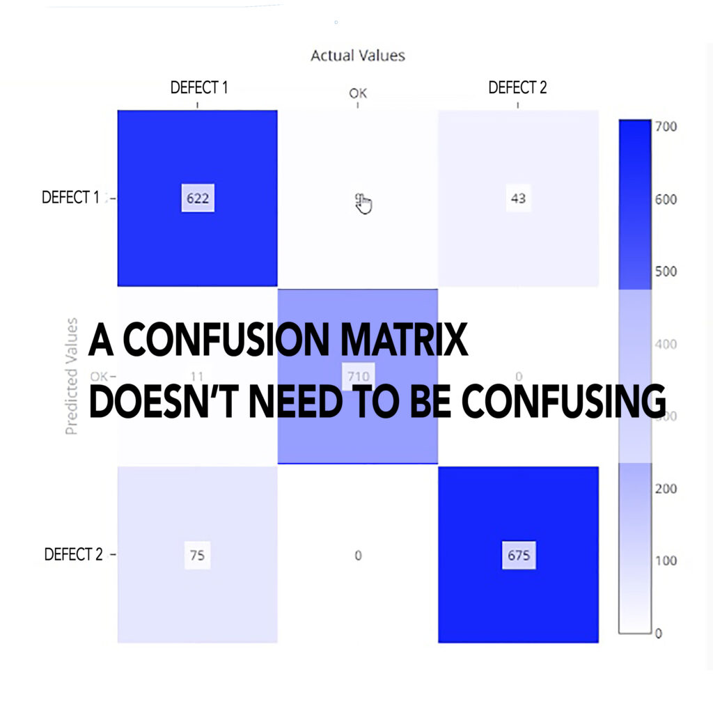
One of the tools we are using to help people address the confusion around model performance is called – somewhat ironically – confusion matrix.
Continue reading the find out what a confusion matrix is and how it can help you assess the performance of an AI model.
What is a Confusion Matrix?
A confusion matrix is a table used to describe the performance of a classification model. It compares the actual target values with those predicted by the model, allowing you to see not just the number of correct predictions but also where the model is making errors.
Let’s get the truly confusing part out of the way first: the positive class in a confusion matrix refers to the class of interest, in QC that are the defective products. The non-defective products are the negatives.
The confusion matrix is structured as follows for a binary classification problem, e.g. whether a product is defective or not.
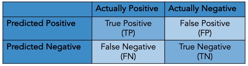
True Positives (TP) are cases where the model correctly predicts the positive class, i.e. defective products which the model categorized as such.
True Negatives (TN) are cases where the model correctly predicts the negative class, i.e. good products which the model categorized as such.
False Positives (FP) are cases where a product is incorrectly identified as defective or failing a quality test when, in fact, it meets all the required standards and specifications. This means that the quality control system mistakenly flags a good product as bad.
False Negatives (FN) are cases where a product is incorrectly identified as passing a quality test and meeting all required standards when, in fact, it has defects or does not meet specifications. This means that the quality control system fails to detect a defective product, allowing it to pass through to the next stage of production.
Key Metrics Derived from a Confusion Matrix
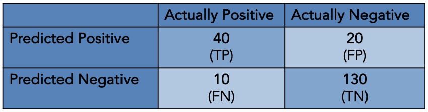
Let’s consider a quality control example like the one mentioned where we have a machine learning model that classifies products into two categories: Positive = defective and negative = good/non-defective.
After running the model on a batch of 200 products and comparing the model’s results to the results obtained by human experts, we get the following confusion matrix:
From these four outcomes, we can derive several key performance metrics. Here is an overview:
- Accuracy: The ratio of correctly predicted instances (both true positives and true negatives) to the total instances. In this case:
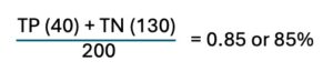 or 85% which means that the model classified 85 out of 100 products correctly – a dismal result for every QC professional but a good example for illustration purposes. It’s also important to consider the distribution of errors (false positives and false negatives) because – depending on the use case – either false negatives or false positive could be a bigger problem for the company.
 - Precision: This metric is used to evaluate the performance of a classification model, specifically focusing on the accuracy of positive predictions. Precision is defined as the ratio of correctly predicted positive instances (true positives) to the total number of instances predicted as positive (both true positives and false positives).Using the table above we get the following calculation:
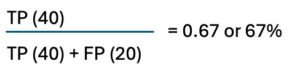 which means that when the model predicts a product as defective it is correct in about 67% of the cases. This metric is important because high precision means that when a product is classified as defective, it is very likely to be genuinely defective. (obviously, the 67% precision in the model scenario is a horribly bad, unacceptable result).
 - Recall, also known as sensitivity, is a metric used to evaluate the performance of a classification model, focusing on the model’s ability to correctly identify all positive instances/defective products. Recall is defined as the ratio of correctly predicted positive instances (TPs) to the total number of actual positive instances (both TPs and FNs).Using the above scenario we get:
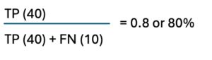 which means the model correctly identifies 80% of all the defective products but it misses 20%products by incorrectly classifying them as good (false negatives).
 - Specificity (or true negative rate) is a metric used to evaluate the performance of a classification model by measuring the proportion of actual negative instances that are correctly identified as negative. Specificity is defined as the ratio of true negatives to the total number of actual negative instances (both TNs and FPs). Using the numbers above we can calculate the specificity:
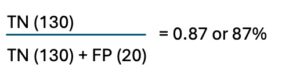 which means that model correctly identifies 87% of the good/non-defective products as non-defective – which would be a completely unacceptable specificity in a manufacturing environs.
Why Use a Confusion Matrix?
The confusion matrix provides a comprehensive view of how well a classification model is performing and can therefore either instill confidence in the results going forward or mean that the model requires additional training and testing – and another confusion matrix after that – to perform well.
Here are some additional reasons why a confusion matrix is valuable:
- Detailed Error Analysis: Unlike simple accuracy, a confusion matrix provides insight into the types of errors your model is making. For instance, high accuracy might mask the fact that your model is not performing well on a particular class.
- Balanced Performance Assessment: Precision and recall derived from the confusion matrix help in understanding the trade-off between false positives and false negatives. This is especially important in applications where the cost of different types of errors varies.
- Easy Interpretation: For stakeholders who may not be familiar with complex metrics, the confusion matrix provides a straightforward way to understand the model’s performance in terms of actual and predicted classifications.
What’s the Confusion About?
Now the name might be a bit confusing, or the matrix itself, but that is not why a confusion matrix is called that. A confusion matrix is called a “confusion matrix” because it provides a detailed breakdown of the performance of a classification algorithm by showing where the model might be “confused.”
Specifically, it displays and categorizes the number of correct and incorrect predictions and highlights instances where the classifier made errors, such as false positives and false negatives thus revealing how the classifier might be “confusing” one class for another.
This detailed insight helps you understand the specific nature and sources of classification errors and points at how to improve the model.
Here are some additional blogs if you are interested in the more technical aspects of AI: